
PID Control Explained: P, I and D Actions, Tuning and Troubleshooting
On this page
PID control is the workhorse of industrial automation. Most flow, pressure, temperature and level loops in a typical process plant use some form of PID algorithm, running in a PLC, DCS or single-loop controller. Understanding what each term does, and how to tune it, is one of the most valuable skills an instrumentation or control engineer can have.
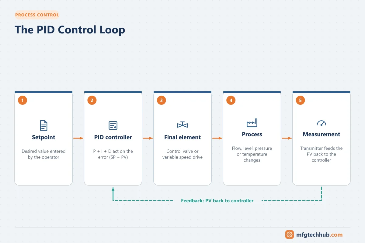
This guide explains PID control from first principles, with practical tuning advice and troubleshooting tips. When you are ready to calculate settings, use our free PID tuning calculator.
The control loop
Every feedback control loop has the same basic parts:
| Element | Role | Example |
|---|---|---|
| Process variable (PV) | The measured value you want to control | Tank temperature |
| Setpoint (SP) | The target value | 80 °C |
| Error (e) | The difference SP − PV (or PV − SP) | 2 °C |
| Controller output (CO or OP) | The signal sent to the final element, usually 0-100% | 45% |
| Final control element | The device that changes the process | Steam control valve |
The controller continuously compares the PV with the setpoint and adjusts its output to reduce the error. PID describes three ways of calculating that output.
Proportional action (P)
Proportional action produces an output proportional to the current error:
P output = Kp × eA large gain (Kp) gives a strong response to a small error. Some controllers use proportional band (PB) instead, where PB % = 100 ÷ Kp. A PB of 50% is the same as a gain of 2.
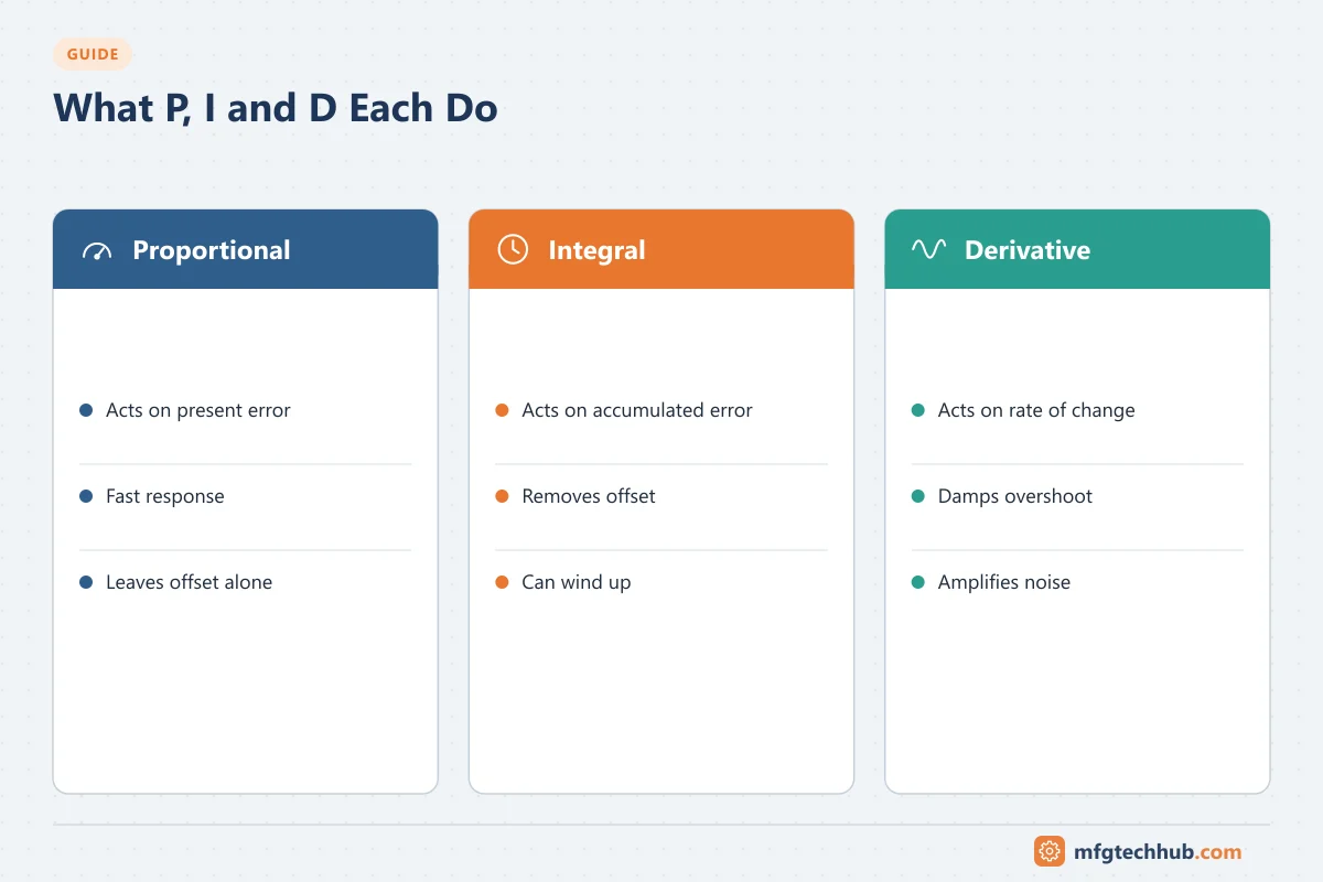
What P does well: it responds immediately to changes.
Its limitation: with proportional action alone, most processes settle with a permanent offset between PV and setpoint. The controller needs some error to produce any change in output, so the error never quite reaches zero. Increasing the gain reduces the offset but eventually makes the loop oscillate.
Integral action (I)
Integral action adds up the error over time:
I output = (Kp ÷ Ti) × ∫ e dtAs long as any error remains, the integral term keeps changing the output. This eliminates offset, which is why almost every industrial loop uses integral action.
The integral time Ti (also called reset time) is expressed in minutes or seconds per repeat. A shorter Ti means stronger integral action. Some controllers use the reciprocal, in repeats per minute.
Its limitation: too much integral action causes slow, rolling oscillation and overshoot. Integral action also causes windup (explained below).
Derivative action (D)
Derivative action responds to the rate of change of the error:
D output = Kp × Td × de/dtIt anticipates where the process is heading and applies a braking effect, which can reduce overshoot and allow faster tuning on slow processes with significant lag, such as temperature loops.
Its limitation: derivative action amplifies measurement noise. On noisy measurements such as flow or level, it usually does more harm than good. Many practitioners leave derivative off unless the loop clearly benefits from it. Where it is used, a derivative filter is normally applied, and derivative is often calculated on the PV rather than the error to avoid a “kick” when the setpoint changes.
Putting it together: the PID equation
In the ideal (ISA standard) form, the three actions combine as:
CO = Kp × [ e + (1/Ti) × ∫ e dt + Td × de/dt ] + bias| Action | Main effect | Too much causes |
|---|---|---|
| P | Fast response, reduces error | Oscillation, noisy output |
| I | Removes offset | Overshoot, slow oscillation, windup |
| D | Reduces overshoot on lagging processes | Output noise, valve wear |
Controller forms
Vendors implement PID in different forms, and settings are not directly interchangeable between them:
- Ideal (standard) form: gain multiplies all three terms, as shown above. Common in modern DCS.
- Series (interacting) form: based on older pneumatic controllers; the P, I and D terms interact.
- Parallel form: independent gains Kp, Ki and Kd. Common in PLC function blocks.
When moving tuning between systems, always check which form, which units (seconds or minutes, gain or PB) and which direction each controller uses.
Direct and reverse action
The controller action must match the process:
- Reverse acting: output decreases when PV rises above setpoint. Example: a heating valve on a temperature loop.
- Direct acting: output increases when PV rises. Example: a cooling valve, or a level loop controlling an outlet valve.
The valve’s fail-safe action (air-to-open or air-to-close) also affects this choice. A loop with the wrong action drives the output to one extreme and is easy to recognize.
Common control loop types and typical settings
| Loop | Typical behavior | Usual controller |
|---|---|---|
| Flow | Fast, noisy | PI with low gain and short integral time |
| Liquid pressure | Fast | PI |
| Gas pressure | Moderate, often integrating | PI, sometimes P-only |
| Level | Integrating (no natural balance) | P or PI; often tuned loosely to absorb surges |
| Temperature | Slow, with dead time and lag | PI or PID |
Level loops deserve special mention. In many plants, a surge tank exists precisely to absorb flow variations. Tuning the level loop “tightly” passes every disturbance on to downstream equipment. Averaging level control, which lets the level move within limits, is often the better choice.
How to tune a PID loop
Before tuning: check the basics
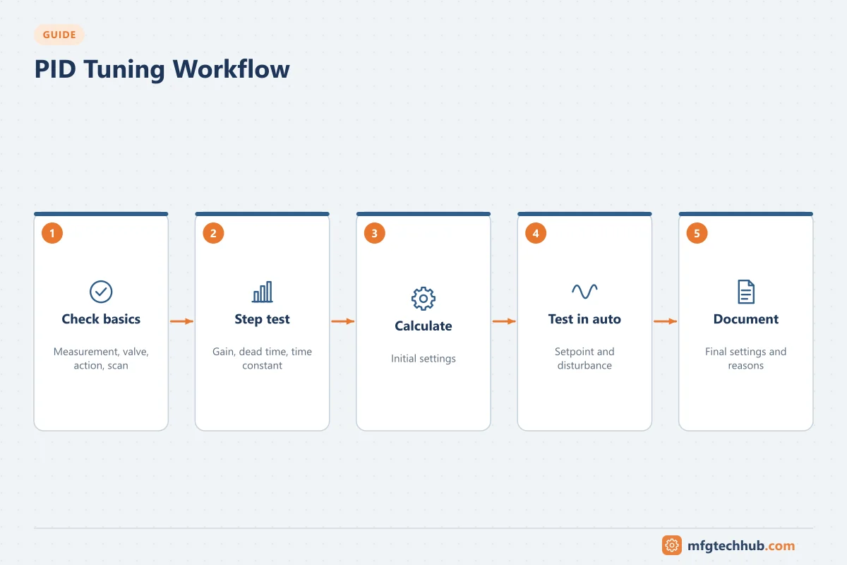
Most “tuning problems” are actually equipment or configuration problems. Check first:
- Measurement: Is the transmitter ranged correctly? Is the signal noisy or frozen? (Our 4-20 mA calculator helps check scaling.)
- Final element: Does the valve move smoothly? Stiction, hysteresis and oversized valves cause oscillation that no tuning can fix.
- Controller action: Is it direct or reverse as required?
- Scan time: Is the controller executing fast enough for the process?
Method 1: Open-loop step test
- Put the controller in manual with the process steady.
- Make a step change in output, for example 5%.
- Record the response and determine the process gain (K), dead time (L) and time constant (T).
- Use tuning rules such as Ziegler-Nichols or lambda tuning to calculate settings.
This method is the safest for most loops because the controller is not in automatic during the test.
Method 2: Closed-loop ultimate gain test
- With integral and derivative action off, increase the gain until the loop oscillates steadily.
- Record the ultimate gain (Ku) and oscillation period (Pu).
- Apply Ziegler-Nichols or Tyreus-Luyben rules.
This test deliberately makes the loop unstable, so only use it where oscillation is safe.
Method 3: Manual (trial-and-error) tuning
Experienced engineers often tune by observation:
- Start with conservative settings: low gain, long integral time, no derivative.
- Increase the gain until the response is reasonably fast without excessive oscillation.
- Reduce the integral time until offset is removed in an acceptable time.
- Add derivative only if the loop is slow and has significant lag.
- Test with small setpoint changes and observe the response to real disturbances.
Whatever the method, make changes in small steps and record the before and after settings.
The PID tuning calculator calculates settings for both test methods, including more conservative alternatives to Ziegler-Nichols.
Troubleshooting common PID problems
The loop oscillates
- Regular oscillation with period similar to the process response: gain too high or integral too strong. Reduce gain first, then lengthen integral time.
- Slow, rolling oscillation: often too much integral action.
- Oscillation with a sawtooth PV and square-ish output: classic sign of valve stiction. Check the valve, not the tuning.
- Oscillation that comes from elsewhere: interacting loops or upstream disturbances. Look at trends of related loops.
Integral windup
When the output saturates at 0% or 100% (for example during startup, or if a valve is too small), the integral term keeps accumulating error. When the PV finally returns, the large stored integral causes a big overshoot. Modern controllers include anti-windup protection, such as stopping integration when the output is at a limit. Make sure it is enabled and the output limits are set correctly.
Noisy controller output
- Remove or reduce derivative action.
- Apply a small filter to the PV (without adding so much lag that control suffers).
- Reduce proportional gain on inherently noisy loops such as flow.
Bump when switching from manual to automatic
Use bumpless transfer, which most controllers support: the setpoint tracks the PV in manual (PV tracking), or the integral term is initialized so the output does not jump.
Beyond basic PID
Single PID loops handle most applications, but some problems need advanced strategies:
- Cascade control: an outer (primary) loop sets the setpoint of a faster inner (secondary) loop, for example temperature cascaded to steam flow.
- Feedforward: measures a disturbance and corrects for it before it affects the PV.
- Ratio control: keeps one flow in proportion to another.
- Split range: one controller drives two valves, such as heating and cooling.
- Override (selector) control: chooses between controllers to protect equipment limits.
These strategies are covered in DCS Control Strategies and illustrated in our boiler drum level control article.
Frequently asked questions
Do I always need all three terms?
No. Most industrial loops use PI control. Derivative helps mainly on slow processes with significant lag, such as many temperature loops.
What is a “good” PID response?
It depends on the process goal. Some loops should respond quickly with a little overshoot; others, such as surge tank levels or loops feeding sensitive equipment, should respond smoothly with no overshoot. Define the goal before tuning.
Why does the same tuning behave differently in two controllers?
The controllers probably use different PID forms, units or scan times. Convert the settings for the target controller’s algorithm.